


We LOVE Excel and Sheets, because it’s almost impossible to imagine doing any SEO tasks without them! From the most basic work to the most complicated, they’re always part of our daily routine. Especially for SEOs, learning advanced formulas is an extra but necessary skill for getting the job done faster. However, as the data grows, even the most logical formula can lose its meaning while you wait for results. (Remember those “Please, don’t crash!” moments staring at the screen?) As a result, working with large websites and more and more data can sometimes turn into chaos. That’s where Python takes the stage: it’s getting more popular every day in the SEO world because of how easy it is to use and what it can do.
In this article, I want to show you how to quickly reproduce the formulas you already use in Excel with Python's Pandas library, using the most basic and simple code. I'll also merge and compare data from the crawl, Google Analytics and Search Console to pull out some useful insights. Don’t worry, learning to code is its own world and a completely different endeavor, but here we’ll just cover the basics: enough code to speed up your daily tasks, which I'll try to pack in generously here, so you save more time. Believe me, it is not that scary! If you want to dig deeper and do more things, check Hamlet Batista’s blog posts about Python and SEO. He rocks! So, those who want to learn new things and save some extra free time, hands up!
Let’s get to work!
Importing Libraries
We will use Pandas for data frames (It is a kind of Excel in Python), Mathplotlib and Seaborn for graphs.
import pandas as pd import numpy as np import matplotlib.pyplot as plt import warnings import seaborn as sns import scipy.stats as stats warnings.filterwarnings('ignore')
Basic Codes to Analyze Crawl Data
Now let’s get the Screaming Frog Crawl data here and read it:
df1 = pd.read_excel('crawl.xlsx',skiprows=1) df1.head()
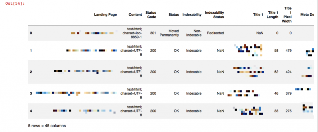
We’ve read our file with pd.read_excel and saved its data in df1. Now df1 has all our crawl data inside. head() just means show me the first 5 rows, which is useful for checking whether our data looks okay. We add skiprows=1 because Screaming Frog’s output does not have column names in the first row; they are in the second row. For example, let's say you want to see your 404 pages and save them in a different file:
df404 = df1[df1['Status Code'] == 404] df404
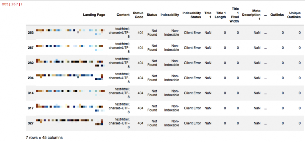
In Python, you need to use ‘==’ to show equality, and ‘!=’ for non-equality. Now I’ll take these 404 pages, put them in another file, and save it:
df404.to_csv('export404.csv', sep='\t', encoding='utf-8')
We exported the pages that gave 404 status codes to the file named export404.csv. Let’s find the pages that don’t have any title tag:
dtitle = df1.loc[df1['Title 1'].isnull()]
isnull() means find those NaN values. We’ve also used .loc here to locate those rows and get them in our output. If you change ‘Title 1’ to ‘Meta Description 1’, then you’ll get pages without meta descriptions. And again, you can save these outputs in csv or excel file just like I’ve shared the “404” example above. If you want to have a quick look for your NaN values, you can use a heatmap and get an overall idea of your data.
plt.figure(figsize=(10,8)) sns.heatmap(df1.isnull(),yticklabels=False,cbar=False,cmap="viridis") plt.show()
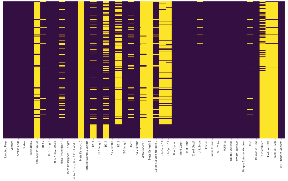
Yellow lines show us NaN values. Let’s see their counts for each column:
df1.isnull().sum()
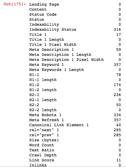
It is that simple, voila! With these basic codes, you can export duplicate pages, redirect pages, pages without title tags and many other crawl outputs into different files, and you can have your crawl outputs ready within seconds in the next crawl just by running these codes.
Merging Crawl Data and Google Analytics Data
Now that you've completed our basic crawl analysis, you'll be able to do some deeper analysis by matching this data to Analytics data.
First, you should get the Landing Page report for the last 1 month or the last 3 months based on the data you want to analyze. I will merge two files by URLs. But first let's read our file as we do in the crawl file:
df_analytics = pd.read_excel('analytics.xlsx') df_analytics.head()
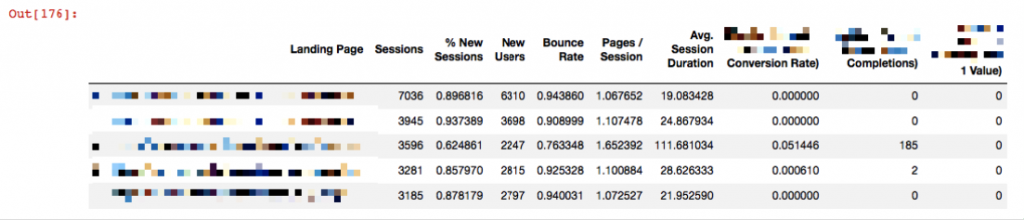
Now it is time to merge them:
merged = pd.merge(df1, df_analytics, left_on='Landing Page', right_on='Landing Page', how='outer') merged.head()
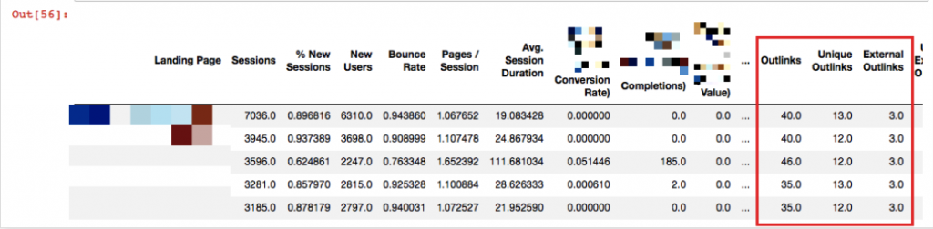
Landing pages have matched with the crawl data.
Crawl Depth Analysis
Screaming Frog gives this graph to us, but it is nice to know how to do this in Python:
plt.figure(figsize=(10,5)) merged['Crawl Depth'].value_counts().sort_values().plot(kind = 'barh') plt.xlabel("URL Counts") plt.ylabel("Crawl Depth") plt.title("Crawl Depth / Pages")
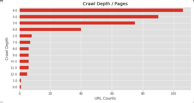
Now, let's approach differently and draw a Session graph against Crawl Depth.
plt.figure(figsize=(10,5))
plt.style.use('ggplot')
plt.bar(merged['Crawl Depth'], merged['Sessions'], color='purple') plt.xlabel("Crawl Depth") plt.ylabel("Sessions") plt.title("Crawl Depth & Sessions")
plt.show()
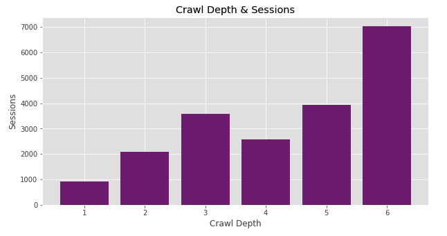
Oops! We encountered an interesting bar chart here. The pages with the high number of sessions appear to be aggregated in Crawl Depth 6! We don’t want our important pages to be accessible by Googlebot after 6 steps. These pages should be more easily accessible and crawled often. Perchance the pages at depth 6 can perform much better, but currently, they are kept pretty far. Check the bar chart below: the OnCrawl study shows that Google is more likely to crawl the pages closer to the homepage.
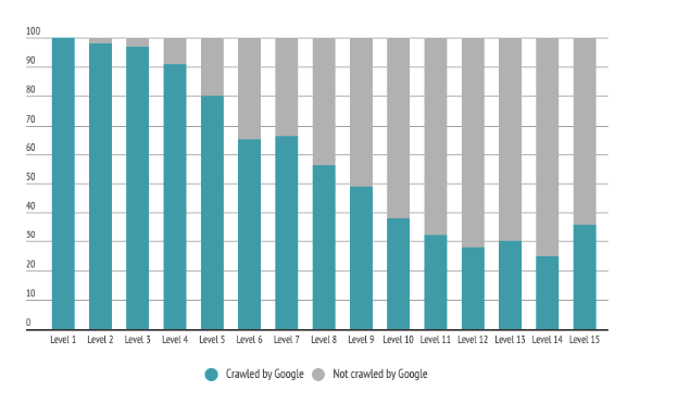
Should we pull these pages forward? Could these be a group of pages or does a single page have a high session, misleading our data? Which other pages do we also have at crawl depth 5?
Questions are leading to more questions and that means one thing: we are on the right track. :) In order to answer these questions, we should analyze our outputs, understand the reasons and, if necessary, take action to bring our important pages forward. Now let's take a look at our pages at Crawl Depth 6:
df_CD6 = merged[merged['Crawl Depth'] == 6] df_CD6.head()
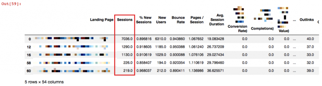
In particular, we should examine the first 3 pages especially, to reduce the crawl depth of them if necessary.
Internal Linking Analysis
Let’s analyze Unique Inlinks also like crawl depth. This time, we will draw a scatter plot to see our in links distribution against ‘’Session’’.
plt.figure(figsize=(15,10)) plt.scatter(merged['Unique Inlinks'], merged['Sessions']) plt.show()
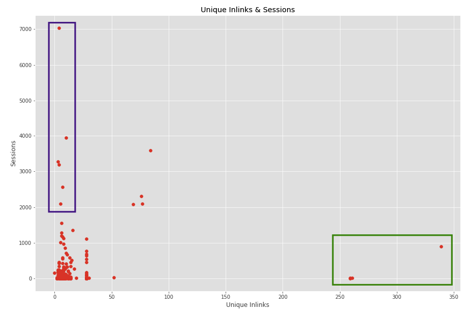
Internal linking is an important factor for the performance of pages. Unnecessarily linking or inadequate linking should be optimized in terms of passing the page value effectively. Let’s look at the graph above. The pages I marked with green on the right side of the plot have a lot of internal links, but not perform very well.
Are these pages really poorly performing pages, do we need to have so many links on these pages, or do they have these links because they are linked from the menu?
In this case, we realized that they are linked from main the menu. Then, you can check whether these pages need to be linked from the menu or not, which is a choice dependant on your strategy. On the other hand, when you look at the pages marked with purple, you’ll see that these pages perform well throughout the site.
However, internal linking does not seem to be sufficient for those. You can obtain these pages and increase their internal linking by finding other relevant pages. Of course, if these pages need optimization. You should also include Search Console data here to be sure. Session data is not enough to decide on action to take but it gives an opinion to analyze deeply.
Response Time Analysis
In order to see how quickly do our pages respond, just draw a histogram of response time.
plt.hist(merged['Response Time'], color = 'green') plt.xlabel("Response Time (seconds)") plt.ylabel("URL Counts") plt.title("Response Time & URL counts") plt.show()
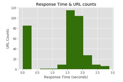
Most of the pages have response time between 1.5-2 seconds which is not good. To optimize it, we can extract pages that respond more than 1.5 seconds and analyze their speed scores with the Pagespeed Insights tool or any other speed tool.
df4 = merged[merged['Response Time'] >= 2.0] df4.head()
Detecting Potential Orphan Pages
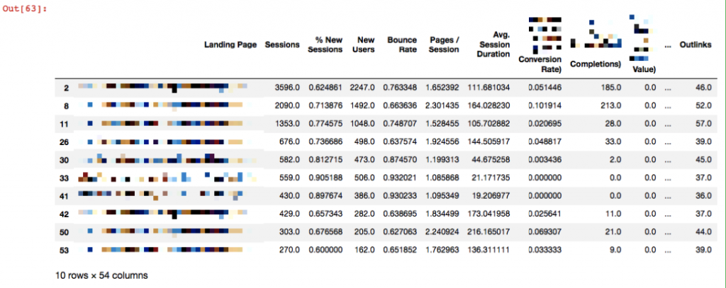
Since I combined Analytics data with crawl data, identifying potential orphan pages is not a big deal. If a page that has Session hits in Analytics does not appear in crawl analysis, this page is either redirected and removed from the site, or it is not linked from anywhere within the site, even if the page is alive.
d_orphan = merged.loc[merged['Status Code'].isnull()] d_orphan
Since each crawled URL will have a status code, the ones that are identified as NaN are the pages coming from the Analytics data.
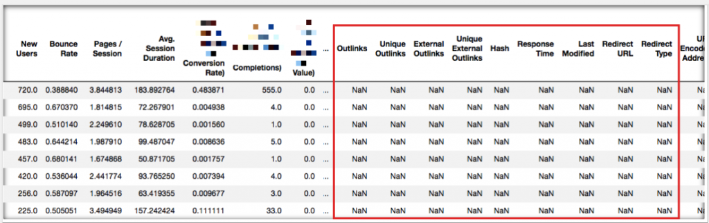
As you can see from the above table above, the pages that are not in the crawl are now detected clearly. Now you can crawl those pages again to see if there are any 200 status codes in them.
Adding A New Column to Dataset & Tag Pages by Grouping Them
Let's say your pages have a specific URL pattern and your goal is to evaluate them by grouping. In my example, these pages will be blog. Since my URLs include /blog/, I'd like to find and group them as blog tag in a new column:
d_blog = merged[merged['Landing Page'].str.contains('^https://www.example.com/blog/')\] d_blog['group'].fillna("blog", inplace = True) d_blog.head()
First of all, you should find your relevant pages including that specific string with str.contains. Then, create the group column. (if you write df[‘example’] and if you don’t have that column in your dataset, it will be created. You don’t need to define it.) Lastly, fillna(‘’blog’’, inplace = True) means write blog to those blank cells and with inplace = True, save the changes.
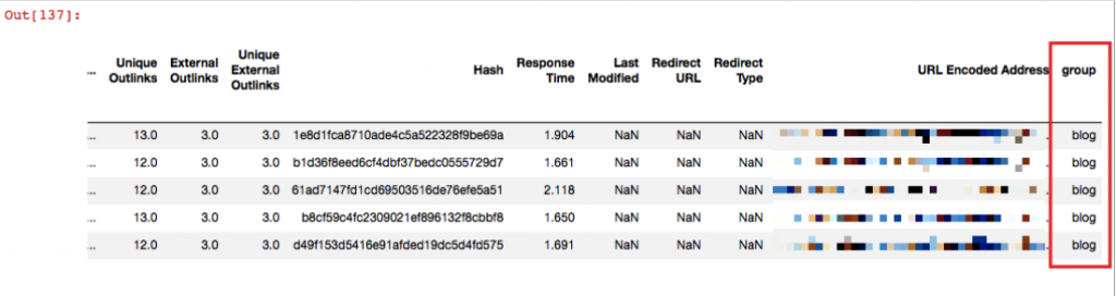
Now you can make groups of your pages and analyze them in terms of ‘’type of page’’.
Adding Search Console Data to Dataset
d_console = pd.read_excel('console.xlsx') merged2 = pd.merge(merged, d_console, left_on='Landing Page', right_on='Landing Page', how='outer') merged2.head()
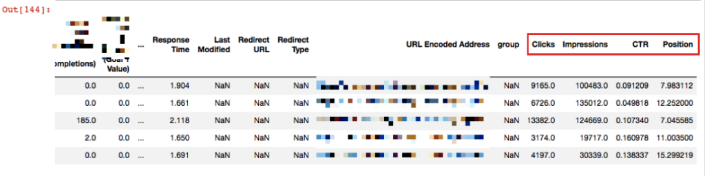
Now I have Console data also in my dataset. Let’s have a quick look for Crawl Depth against Position:
plt.figure(figsize=(10,5))
plt.style.use('ggplot')
plt.bar(merged2['Crawl Depth'], merged2['Position'], color='purple') plt.xlabel("Crawl Depth") plt.ylabel("Position") plt.title("Crawl Depth & Position")
plt.show()
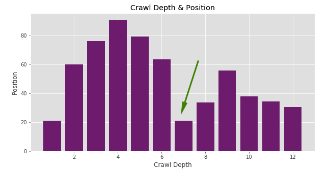
For example, you can see a number of pages in Crawl Depth 7 that have an average position of 20 in all the queries that pages get impressions. There is a possibility for optimization. Due to the “Position” data, I can assume there are some potential pages to optimize and I can see the effect quicker.
However, the “average position” data may not always guide you correctly. Here, it will be much more accurate to analyze the keywords all together.
Word Cloud Graph
This is a graph to quickly identify word density in a dataset. You can use it for anchor texts or the titles of a particular group of pages. Let’s see a code example from a different dataset and its graph:
# öncelikle wordcloud kütüphanesini import ediyoruz
from wordcloud import WordCloud
harvard = df[df['Institution'] == 'HarvardX']
wordcloud = WordCloud(background_color="white").generate(" ".join(harvard["Course Subject"])) plt.figure(figsize=(10,5)) plt.imshow(wordcloud, interpolation='bilinear') plt.axis("off")
plt.show()
 To summarize... As you can see, we are able to do a lot of analysis with some basic and similar codes. You can quickly analyze your data by only learning these simple ones. In fact, you don’t need to have a large pool of data to use Python. You may have noticed that we quickly got some insights by simply creating graphs with just a couple of lines of codes.
When you do this by working on Excel or Google Sheets, you'll need to invest in more time. If you can’t find related codes similar to the examples above or you simply want to work on different things, please let me know in the comment section below. If you are shy to drop a comment, you will definitely find your answers on sites like Stackoverflow.


